Benchmarks | Compare Ingrid Cloud with real life measurements

Benchmarks
You can trust Ingrid Cloud

Ingrid Cloud's simulation results have been thoroughly compared to wind tunnel measurements in various benchmark cases. With our automated mesh generation technology, we have continuously delivered accurate results and outperformed our competitors.

Ingrid Cloud's score sheet

80% Accuracy
For turbulence sound
97% reduction in total simulation time
84% lower cost compared to a large competitor

Background

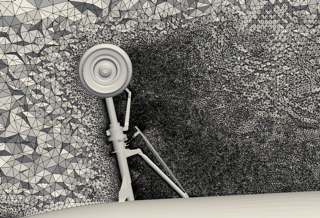
This NASA/AIAA benchmark presents a direct comparison of simulation results obtained using Ingrid Cloud’s intelligent algorithm with wind tunnel measurements on a Gulfstream G550 nose landing gear Figure 1 The objective was to assess the accuracy of Ingrid Cloud’s solver when predicting turbulent flow and noise generation by the landing gear of an aircraft approaching landing. The experimental work was carried out by researchers from the NASA Langley Research Center [1] and provided a series of detailed, well-documented wind tunnel measurements for comparison and validation of simulation results.

The surface mesh in Figure 1 clearly illustrates how we create the “initial guess” volume mesh. On the one hand, the surface of the landing gear is accurately represented in its finest details. On the other hand, the mesh is dramatically coarser close to wind tunnel walls, away from the landing gear (with cell sizes that are as large as the wheels themselves). This way, we leave the decision of where to refine the volume mesh to Ingrid Cloud’s intelligent algorithm, which will then produce a fine mesh based on the choice of output. In this problem, the output chosen was the turbulent sound generated by the landing gear.

Figure 1
image

Surface mesh (left) and “initial guess” volume mesh (right). For the computations, we fed the “initial guess” volume mesh into Ingrid Cloud’s intelligent algorithm so that it could perform automatic mesh refinement and compute sound sources originated when an aircraft approaches landing.

Method

This problem was solved in a one way, uncoupled system of equations, where incompressible Navier-Stokes equations were solved to compute the flow and a wave propagation problem was solved to compute sound. Both equations are complemented by their continuous adjoint equations and their solutions are used, together with other heuristics, to compute error estimations and refine the mesh.

For this benchmark, the refinement goal was the sound sources of Lighthill’s wave equation [2]. Both fluid and sound problems were solved simultaneously on the same mesh to avoid I/O and interpolation issues; the supercomputer “Beskow” at PDC Center for High Performance Computing in Stockholm was used.

Results

Below Figure 2 shows the volume mesh for different levels of refinement. The finest mesh is clearly more refined in the wake of the gear (the flow is from left to right) and refinement is performed so that the flow structures important for computation of sound are correctly resolved, leaving other areas unrefined.

Figure 2
image
image
image

Volume mesh refined by Ingrid Cloud from “initial guess” (left) to final mesh (right). The adaptive algorithm is an iterative process where several iterations are performed before the final mesh is obtained. Here, only 3 iterations are shown for simplicity.

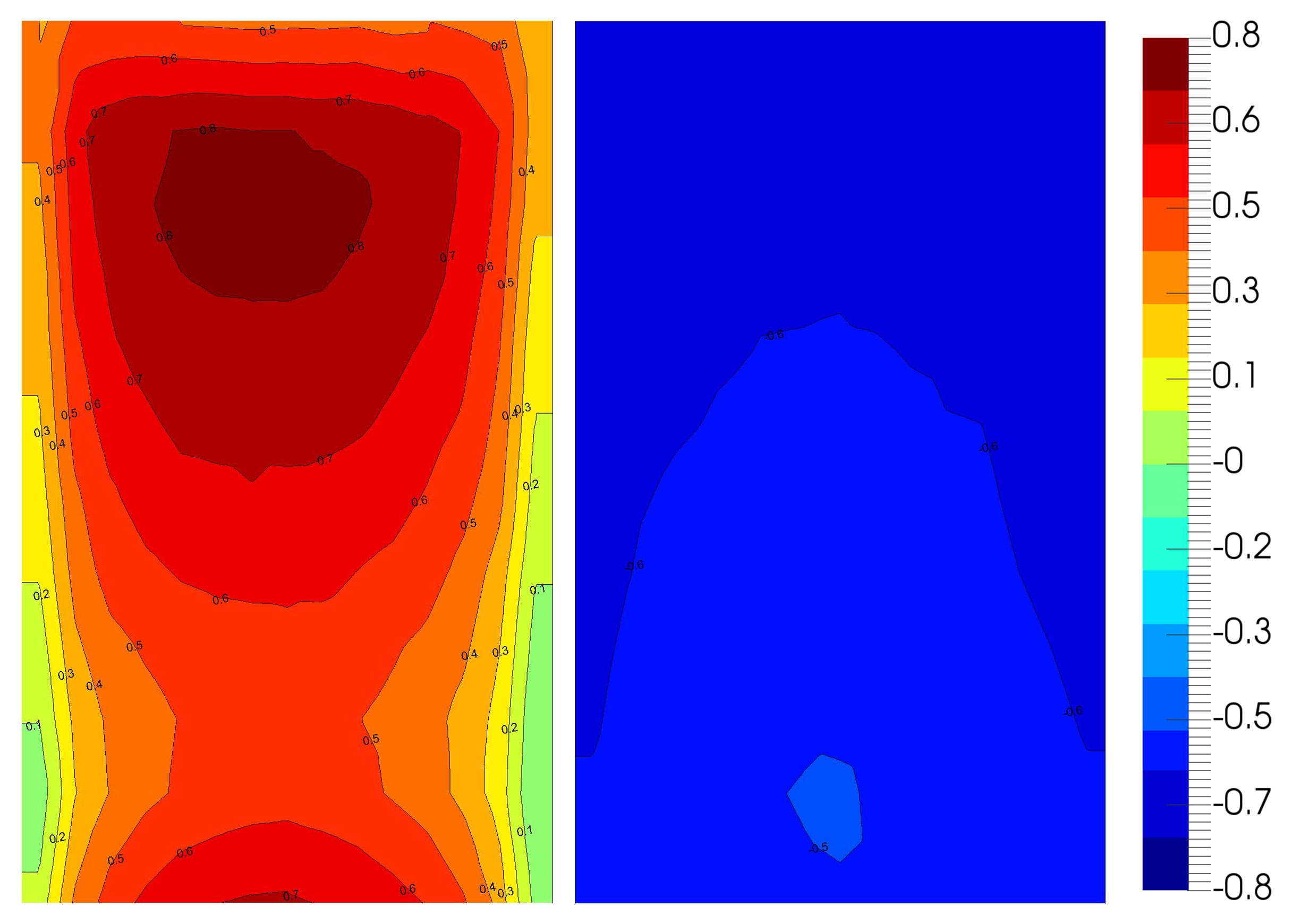
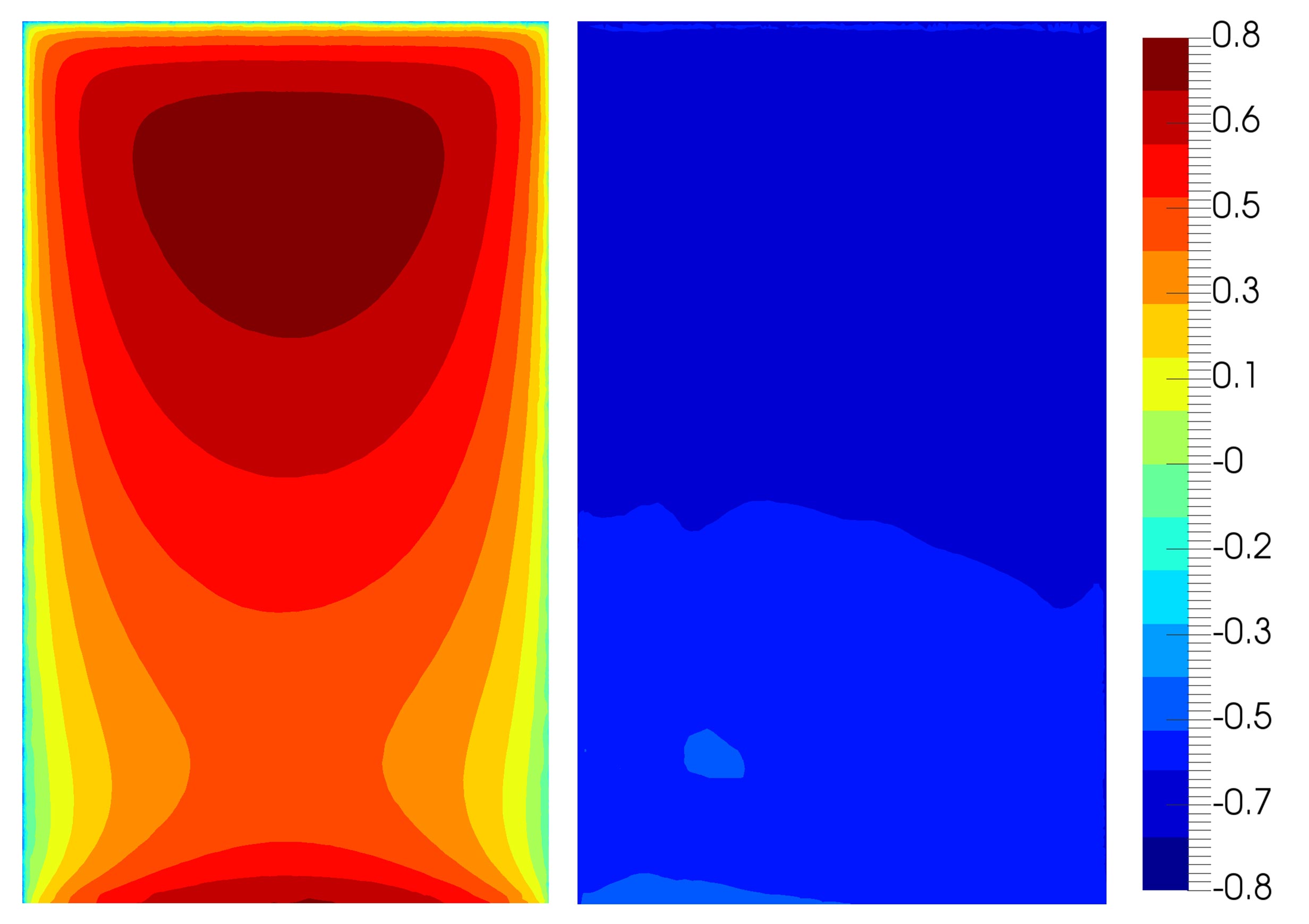
Below Figure 3 brings an overview comparison with wind tunnel PIV plane measurements, where time-averaged contours of streamwise velocity, 2D turbulent kinetic energy (TKE) and Z-vorticity are shown; the quantities were plotted on two planes, one passing through the starboard wheel and the other through the wake of the landing gear door.

There is a good qualitative agreement between experiments and simulation. One remarkable feature of the comparison is that there is a clear asymmetry between the port and starboard sides when observing the door plane, both in the streamwise velocity and TKE fields. This is not an intuitive result; however, a closer look at the geometry reveals that the landing gear is indeed asymmetrical with respect to its longitudinal plane. The adaptive mesh refinement automatically captures this behaviour, which would be a somewhat intricate task had we generated and refined the mesh manually.

Another interesting feature of the comparison is that we apparently get an overshoot of vorticity on the side of the starboard wheel; this is probably due to the low resolution of the PIV measurement as compared to the resolution of the computational mesh, and not an “overshoot”: the wheels constitute a strong source of unsteadiness and we expect the mesh refinement to capture this behaviour, producing a fine mesh in that area. The PIV resolution is 1.3 mm [1] and the computational mesh close to the wheels is smaller than 1.3 mm on several cells coinciding with the region of strongest vorticity.

Figure 3
image

PIV, location of measurement planes; time-averaged fields of streamwise velocity, 2D turbulent kinetic energy and vorticity. In all figures: left, simulation, right, measurements [11].

Sound pressure levels were measured at 20 different locations at the University of Florida Aeroacoustic Flow Facility (UFAFF), Figure 4. A selection of 6 representative microphones is compared with measured values in Figure 5. The signals compare well, especially in the frequency range of 800–2000 Hz for the flyover microphones, and 1000–9000 Hz for the sideline ones. The sideline microphones show, in general, better agreement, which may be a consequence of lack of resolution in the mesh, causing dispersion of waves as they travel a longer distance (flyover microphones are ca. 1 m further away from the gear than sideline ones).

Figure 4
image

Microphone locations in the UFAFF wind tunnel.

Figure 5
image

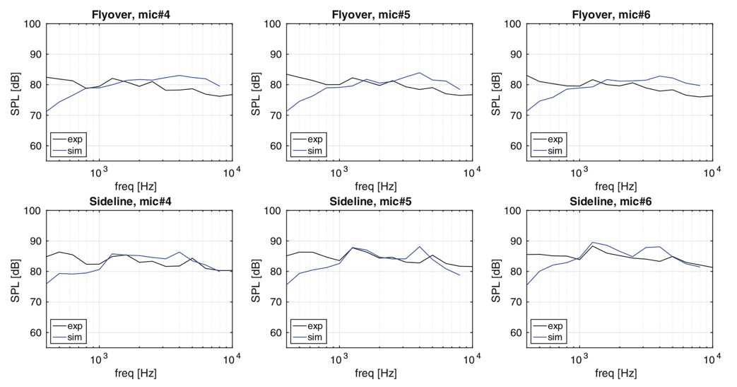
Comparison of Sound Pressure Level (SPL) for selected microphones.

Finally, Figure 6 shows a comparison of the integrated error of the sound pressure levels in all microphones between Ingrid Cloud’s computations and the computations performed by a direct competitor. Thanks to its intelligent algorithms, Ingrid Cloud largely outperforms the competitor’s computations.

Figure 6
image

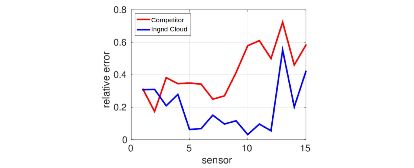
Comparison of integrated error in all microphones, showing that Ingrid Cloud outperforms a major competitor.

References

[1] Neuhart DH et al (2009), Aerodynamics of a gulfstream g550 nose landing gear model, In Proceedings for the 15th AIAA/CEAS Aeroacoustics Conference (30th AIAA Aeroacoustics Conference).

[2] Vilela de Abreu R et al (2011), Adaptive computation of aeroacoustic sources for a rudimentary landing gear using Lighthill’s analogy, In Proceedings for the 17th AIAA/CEAS Aeroacoustics Conference (32nd AIAA Aeroacoustics Conference).

Links

http://...
http://...


Ingrid Cloud's score sheet

95% Accuracy
For wind at pedestrian height
97% reduction in total simulation time
84% lower cost compared to a large competitor

Background

This benchmark was proposed by the Architectural Institute of Japan (AIJ) for validation of CFD codes when used for the computation of flow around buildings and city areas. All cases were measured in a wind tunnel and offer a reliable way for validation of simulation codes [1].

Using Ingrid Cloud, we computed solutions to three of the AIJ benchmark cases, each one with an increasing complexity of geometry Figure 1. Case A models the flow past a simple geometry representing a building; Case D models a high-rise building surrounded by a group of smaller buildings; and Case E is a reduced scale model of a neighborhood in the city of Niigata in Japan. Our results were presented at the ECCM-ECFD 2018 in Glasgow, Scotland (a joint conference between the 6th European Conference on Computational Mechanics and the 7th European Conference on Computational Fluid Dynamics).

Figure 1
image
image
image

The three AIJ benchmark problems (Case A, D, E) used in the validation of Ingrid Cloud for flow in urban areas.

Method

This problem was solved using Ingrid Cloud’s unique intelligent algorithm to refine the mesh and compute the turbulent flow solutions. For all cases, the refinement goal was to model the wind pressure forces acting on the buildings. The only input parameters were geometry and wind velocity (magnitude and direction).

The problem was solved with the supercomputer Beskow at PDC Center for High Performance Computing in Stockholm. Boundary conditions were specified according to the guidelines in [1] and are the same boundary conditions implemented in the Urban Wind Comfort and Building Wind Load apps.

Results

Below Figure 2 shows the volume mesh for different levels of refinement for the city of Niigata (Case E) together with a snapshot of a flow field for each refinement level. As the mesh is refined, more turbulent structures are revealed in the wake of the high-rise building. This is a unique feature of Ingrid Cloud, where the user just needs to input wind velocity and geometry and Ingrid Cloud will generate and refine the mesh.

For Case A, we show the results in Figure 3. The wind tunnel measurements available were wind velocities at selected points in the wake of the building/box. The agreement is nothing short than excellent and can be summarized by the Pearson correlation coefficient between measured and simulated velocities – which for this case was r=0.94 (r=1 means full agreement between wind tunnel and simulation). For Case D Figure 4 the Pearson correlation is r=0.83 and for Case E Figure 5, r=0.75.

As observed, the more complex the problem, the worse the correlation between wind tunnel and simulation. However, a Pearson coefficient of 0.75, as obtained for the city of Niigata (Case E), is a very good result: if one computes the average error between wind tunnel and simulation data, the result is 4.5%. Finally, we need to keep in mind that wind tunnels are also an approximation of reality, where flow scales are much larger than the scales that can be achieved in a wind tunnel.

Figure 2
image
image
image
image
image
image

Overview of mesh refinement. Instantaneous wind speed for different levels of automated mesh refinement using Ingrid Cloud (flow from left to right). As the mesh is refined, more flow structures are revealed in the solution. On the right, the finest mesh shows clearly that the refinement acts more intensively in the wake of the high-rise building.

Figure 3
image
image

Case A. Comparison of wind speed for all measurement points (left). The Pearson correlation coefficient is 0.94.

Figure 4
image
image

Case D. Comparison of wind speed for all measurement points. The Pearson correlation coefficient is 0.83.

Figure 5
image
image

Case E. Comparison of wind speed for all measurement points. The Pearson correlation coefficient is 0.75.

References

[1] Tominagaa, Y., et al (2008), “AIJ guidelines for practical applications of CFD to pedestrian wind environment around buildings”, Journal of Wind Engineering and Industrial Aerodynamics, vol. 96, 1749–1761.

Media


Ingrid Cloud's score sheet

83% Accuracy
For surface pressure
97% reduction in total simulation time
84% lower cost compared to a large competitor

Background

This benchmark illustrates how accurately Ingrid Cloud can compute aerodynamic forces on high-rise buildings. We have used Ingrid Cloud to simulate wind flow past the geometry of a high-rise building that had been tested in a wind tunnel facility before and obtained more than a 99% correlation between measured and computed surface pressure distribution. The geometry is a part of an open aerodynamic database created by tokyo Polytechnic University [1].

Method

For this benchmark, Ingrid Cloud used the surface pressure distribution as the refinement target for its adaptive algorithm. This is the same refinement target implemented in the Building Wind Load app. Figure 1 shows the coarsest mesh, (which is used as an input to Ingrid Cloud), and the resulting finest mesh.

Computations were performed on supercomputer Hazel Hen, a Cray XC40 system located at the High-Performance Computing Center Stuttgart (HLRS). With a peak performance of 7.42 Petaflops (quadrillion floating point operations per second), Hazel Hen is one of the most powerful supercomputers in the world (position 27 in the TOP500, July 2018) [2]. Hazel Hen is one of several ultramodern supercomputers available in Ingrid Cloud.

Figure 1
image
image
image
image

Overview of flow velocity on a coarse mesh and on the finest mesh automatically created by Ingrid Cloud.

Results

Time-averaged pressure coefficients were measured using pressure taps on the surface of the building. Over 400 sensors were used. The Pearson correlation coefficient between Ingrid Cloud and measured values obtained was 0.995. A comparison is shown in Figure 2.

Figure 2
image

Comparison of pressure coefficients. The Pearson’s correlation coefficient is 0.995.

Pressure Coefficient, Surfaces. For both windward and leeward. A comparison between a wind tunnel and Ingrid Cloud is shown in Figure 3.

Figure 3
image

WIND TUNNEL: Windward (left) & Leeward (right)

image

INGRID CLOUD: Windward (left) & Leeward (right)

References

[1] http://www.wind.arch.tkougei.ac.jp/info_center/windpressure/highrise/Homepage/homepageHDF.htm

[2] https://www.hlrs.de/systems/cray-xc40-hazel-hen/

Links

http://...
http://...